Quick start

Almost all interaction with pygeosolve is made through the Problem object:

from pygeosolve import Problem

# Create a new problem.
problem = Problem()

Adding primitives

The currently available geometric primitives are Line and Point. These can be added to the problem using Problem.add_line() and Problem.add_point(), respectively.

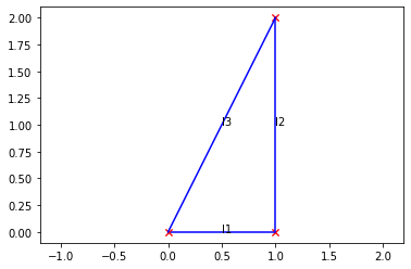
Let’s create a triangle from three lines, starting with the first:

problem.add_line("l1", (0, 0), (1, 0))

The first argument is a unique name to give to the primitive. Lines additionally take two points - their start and end - as arguments.

We want the second line’s start point to share the first’s end point, and the third line’s start to connect the end of the second line to the start of the first. We can do this by referencing the existing lines’ points in the new lines using Problem’s dict-like access:

problem.add_line("l2", problem["l1"].end, (1, 2))
problem.add_line("l3", problem["l2"].end, problem["l1"].start)

We’ve made a right triangle:

problem.plot()

Adding constraints

Let’s try to make the triangle equilateral. We can do this by constraining the lines. We’ll do this by constraining all of the line lengths to be equal, for which equilateral triangle are the only solutions. An alternative would be to constrain the angles between the lines at each vertex to be ±120°.

Problem providesd methods to fix the position of a line (Problem.constrain_position()), set the length of a line (Problem.constrain_line_length()), and set the angle between two lines (Problem.constrain_angle_between_lines()). The primitive(s) referenced by each call have to already exist in the problem.

Let’s fix the position of l1 and constrain the length of l2 and l3 to that of l1:

# Fix l1 in its current position.
problem.constrain_position("l1")

# Constrain the lengths of l2 and l3 to be the same as that of l1.
problem.constrain_line_length("l2", problem["l1"].length())
problem.constrain_line_length("l3", problem["l1"].length())

The status of the current problem can be printed with str():

print(str(problem))

Problem with 2 free parameter(s):
    Line(l1, [Point(__l1_p0__, (0, 0)), Point(__l1_p1__, (1, 0))], length=1.0, angle=90.0)
    Line(l2, [Point(__l1_p1__, (1, 0)), Point(__l2_p1__, (1, 2))], length=2.0, angle=0.0)
    Line(l3, [Point(__l2_p1__, (1, 2)), Point(__l1_p0__, (0, 0))], length=2.23606797749979, angle=-153.434948822922)
and 2 constraint(s):
    LineLengthConstraint(current=2.0, error=1.0)
    LineLengthConstraint(current=2.23606797749979, error=1.5278640450004208)

    Total error: 2.527864045000421

Solving

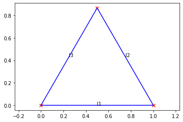
At this point our problem can be solved by calling Problem.solve():

result = problem.solve()
problem.plot()

The return value contain information about the solution. If no solution was found, its success attribute will be False:

print("Success:", result.success)
print("Number of cost function evaluations:", result.nfev)

Success: True
Number of cost function evaluations: 2109

Let’s check the lengths and angles are as they should be:

print(problem["l1"].length())
print(problem["l2"].length())
print(problem["l3"].length())
print(problem["l1"].angle_to(problem["l2"]))
print(problem["l2"].angle_to(problem["l3"]))
print(problem["l3"].angle_to(problem["l1"]))

1.0
0.999999998993984
1.0000000057925704
-119.99999958348788
-120.00000015833795
-120.00000025817418

Sometimes the solution to the above problem switches between angles with +120° and -120°. This is because both angles are solutions to the given constraints. The solver performs a stochastic optimisation that may happen to settle upon a solution with a particular sign. The chosen solution is more likely to resemble the initial positions of the points. If you want to make it more likely a particular solution is the one chosen, draw the initial points close to the expected result. For example, placing l2’s end point on the negative y-axis will likely lead to a solution with positive angles:

from pygeosolve import Problem

problem = Problem()
problem.add_line("l1", (0, 0), (1, 0))
problem.add_line("l2", problem["l1"].end, (1, -2))
problem.add_line("l3", problem["l2"].end, problem["l1"].start)

# Fix l1 in its current position, and the line lengths to be equal.
problem.constrain_position("l1")
problem.constrain_line_length("l2", problem["l1"].length())
problem.constrain_line_length("l3", problem["l1"].length())

# Solve.
problem.solve()
problem.plot()

# Print lengths and angles.
print(problem["l1"].length())
print(problem["l2"].length())
print(problem["l3"].length())
print(problem["l1"].angle_to(problem["l2"]))
print(problem["l2"].angle_to(problem["l3"]))
print(problem["l3"].angle_to(problem["l1"]))

1.0
0.9999999987394652
0.9999999953284268
120.00000026737064
119.99999980376742
119.99999992886194

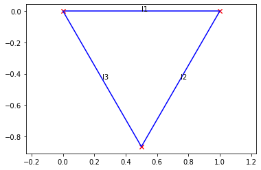
We can force negative angles by constraining the problem in a way that will guarantee the selection of negative angles, such as by requiring them with Problem.constrain_angle_between_lines(). Pygeosolve uses a right-handed coordinate system so positive angles are clockwise. That means if we want the vertex between l2 and l3 to be above l1, we need to constrain the angles to be negative:

from pygeosolve import Problem

problem = Problem()
problem.add_line("l1", (0, 0), (1, 0))
problem.add_line("l2", problem["l1"].end, (1, 2))
problem.add_line("l3", problem["l2"].end, problem["l1"].start)

# Fix l1 in its current position.
problem.constrain_position("l1")

# Constrain the angles between the lines to be -120°.
problem.constrain_angle_between_lines("l1", "l2", -120)
problem.constrain_angle_between_lines("l2", "l3", -120)

# Solve.
problem.solve()
problem.plot()

# Print lengths and angles.
print(problem["l1"].length())
print(problem["l2"].length())
print(problem["l3"].length())
print(problem["l1"].angle_to(problem["l2"]))
print(problem["l2"].angle_to(problem["l3"]))
print(problem["l3"].angle_to(problem["l1"]))

1.0
0.9999999928213432
0.9999999785975914
-120.00000117850392
-119.99999905454597
-119.99999976695014